Metric Decomposition

In this page, we first provide the proof for the metric decomposition used in the paper, and we define Compound Decomposable Metrics for more complex metrics.

Decomposable Metrics

Below, for a complex vision task, \(\mathbf{V}\), that can be represented as a sequential composition of the subtasks, i.e., \(\mathbf{V} = \mathbf{v}_n \odot ...\mathbf{v}_2 \odot \mathbf{v}_1\), we remind the metric compositionality definition.

\(M_\mathbf{V} = F(M^{'}_\mathbf{V}) \text{, where } M^{'}_\mathbf{V} = \prod_{i=1}^{N}{m_{\mathbf{v}_i}}\),

where \(M^{'}_\mathbf{V}\) is a directly decomposable metric of the task \(\mathbf{V}\), \(m_{\mathbf{v}_i}\) is a metric of the i-th subtask, and \(F\) is a monotonic function.

Performance metric AP

The performance of an MVC or a human on a given vision task is usually evaluated using task-specific performance metrics. For the complex vision tasks object detection (\(\mathbf{V}_D\)) and instance segmentation (\(\mathbf{V}_I\)) used in the paper, a commonly used performance metric is Average textit{Precision} (AP) measured for each object class. Each AP of a class is calculated by taking the area under the curve (AuC) of a Precision-Recall curve (PR-curve). The PR-curve is obtained as follows. For each \(\delta\in[0, 1]\), first collect all output bounding boxes with confidence score below \(\delta\); then calculate the precision of these boxes as \(\frac{TP}{TP+FP}\) and recall as \(\frac{TP}{TP+FN}\), where TP is true positive, FP is false positive and FN is false negative. Finally, each pair of (precision, recall) value becomes a point on the PR-curve. A threshold of intersection over union (IoU), usually predefined (e.g., \(0.5\)), is used to determine whether the predicted boundary of the object overlaps with the ground truth enough to be considered a true positive over a false positive. For example, for a predicted bounding box of a bus \(b\) and a ground truth bounding box \(b_0\), \(b\) is considered a true positive if \(IoU(b, b_0) \geq 0.5\) and false positive otherwise. However, calculating precision and recall for each \(\delta\in[0, 1]\) can be expensive; therefore, in practice, a \(\delta\) value is only selected if there exists at least one bounding box with the confidence score that equals to \(\delta\). The procedure for calculating AP for instance segmentation is the same as that for object detection, except each point on the PR-curve is obtained with precision and recall values with the areas enclosed in the outlines rather than bounding boxes.

Decomposition of AP

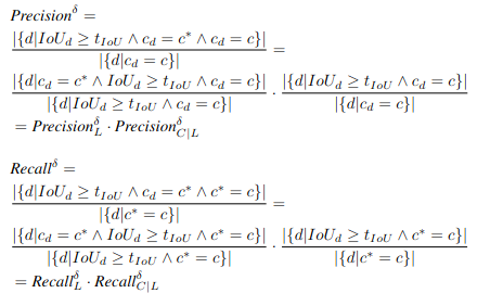
Below, we show that AP is decomposable. First, AP for a class \(c\) is the AuC of the PR-curve. Therefore, by the definition of decomposable metrics, if each PR-curve is directly decomposable, AP is decomposable. Each point on the PR-curve is defined with precision and recall for a class label \(c\) given a \(\delta\) and a IoU threshold \(t_{IoU}\). For object detection, for all detected objects \(d\) such that the confidence score conf\(_d \geq \delta\), where \(c^*\) represents the ground truth class and \(IoU_d\) is the max \(IoU\) of the bounding box compared to all ground truth boxes, we can represent Precision and Recall as: Precision\(^{\delta} = \frac{|\{d|IoU_d \geq t_{IoU}\land c_d = c^*\}|}{|\{d|c_d = c\}|}\) Recall\(^{\delta} = \frac{|\{d|IoU_d \geq t_{IoU} \land c_d = c^*\}|}{\{d|c^* = c\}|}\) .

Thus, Precision\(^{\delta}\) and Recall\(^{\delta}\) can be decomposed as follows:

Note that \(IoU_d \geq t_{IoU} \land c_d = c^*\) is the condition for a detection \(d\) to be a true positive. We can see that for Precision\(^{\delta}\), \(\frac{|\{d|IoU_d \geq t_{IoU}\land c_d = c\}|}{|\{d|c_d = c\}|}\) is the percentage of bounding boxes matched ground truth out of all output boxes of this class, which is precision for \(\mathbf{v}_L\); \(\frac{|\{d|c_d = c^* \land IoU_d \geq t_{IoU} \land c_d = c\}|}{|\{d|IoU_d \geq t_{IoU}\land c_d = c\}|}\) is the percentage of correct labels out of all bounding boxes matched ground truth of this class, which is precision for \(\mathbf{v}_{C|L}\). Similarly for Recall\(^{\delta}\), \(\frac{|\{d|IoU_d \geq t_{IoU}\land c^* = c\}|}{|\{d|c^* = c\}|}\) is recall for \(\mathbf{v}_L\) and \(\frac{|\{d|IoU_d \geq t_{IoU}\land c^* = c\}|}{|\{d|c^* = c\}|}\) is recall for \(\mathbf{v}_{C|L}\). Since both Precision\(^{\delta}\) and Recall\(^{\delta}\) are decomposable, each point on the PR-curve is decomposable, the PR-curve for each class \(c\) can be decomposed into the two subtasks, i.e., PR\(_D =\) PR\(_L \cdot \textit{PR}_{C|L}\). As a result, AP for object detection is decomposable following Metric Decomposition.

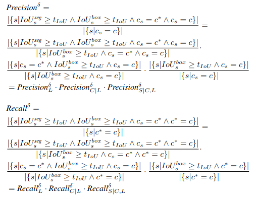
Similarly, AP for instance segmentation is decomposable because we can decompose Precision\(^{\delta}\) and Recall\(^{\delta}\). For a segmented object \(s\), let \(IoU^{\textit{seg}}_s\) be the max \(IoU\) of the area enclosed by \(o_s\) compared to all ground truth segmentation, \(IoU^{box}_s\) be the max \(IoU\) of \(b_s\) compared to all tight bounding boxes around areas enclosed by ground truth segmentation. Precision\(^{\delta}\) and Recall\(^{\delta}\) can be decomposed as the following:

Following the decomposition of Precision\(^{\delta}\) and Recall \(^{\delta}\), we can decompose PR-curves for instance segmentation, i.e., PR\(_I =\) PR\(_L \cdot\) PR \(_{C|L}\cdot\) PR \(_{S|C,L}\). AP used for instance segmentation can also be decomposed following Metric Decomposition.

Compound Decomposable Metrics

Some metrics, such as mean Average Precision (mAP), are more complex and are not decomposable according to our decomposition definition. mAP is defined as an average of AP for each class label c; therefore, mAP can be represented as a function of the precision-recall curve, PR, that is directly decomposable. For such metrics \(M_\mathbf{V}\), we extend the decomposable metric definition into compound decomposable as follows:

\(M_\mathbf{V} = F(M_\mathbf{V}^{1}, ..., M_\mathbf{V}^{K})\text{, where }M_\mathbf{V}^k = \prod_{i=1}^{N_k}\),

where \(M_\mathbf{V}^k\) is a decomposable metric of the task \(\mathbf{V}\), \(m^k_{\mathbf{v}_i}\) is a metric of the i-th subtask, and \(F\) is a function that is monotonic with respect to every argument.

Now we show that mAP is decomposable. Given all class labels \(\mathbf{C}\), mAP is the average of each AP value of \(c\in \mathbf{C}\). Since AP for each \(c\) is decomposable as we showed above, mAP is also decomposable: mAP\(_{\mathbf{V}} = mean(\) AP \(^1, ...,\) AP \(^{|\mathbf{C}|})\).